How to Process Nebula using Pixinsight
Processing is a big part of Astro Photography. It is all good to collect all this data, but poor processing reduces the chance of picture quality. Like all things with processing, it is a personal preference to how you like the picture. Your preferences may change over time, but nevertheless, it still is your preference that matters.
This page will show you the process I take with processing Nebula in Pixinsight and list all the add-ons I use. Remember the process is just as important as the pictures, don’t skimp on purchasing decent processing software and add-ons. You spend thousands on AP equipment and a few hundred on processing software is an easy decision. Which software is down to you of course. This is a more beginner version designed for people who have never used it or are just in the beginning stages of using Pixinsight.
Software and add-ons used, price and links:
Apart from DSS, all the add-ons above are used in PI. The other potential software is Topaz Denoise - https://www.topazlabs.com/denoise-ai. This is a stand-alone software, but I have no experience with this software.
Processing is a big part of Astro Photography. It is all good to collect all this data, but poor processing reduces the chance of picture quality. Like all things with processing, it is a personal preference to how you like the picture. Your preferences may change over time, but nevertheless, it still is your preference that matters.
This page will show you the process I take with processing Nebula in Pixinsight and list all the add-ons I use. Remember the process is just as important as the pictures, don’t skimp on purchasing decent processing software and add-ons. You spend thousands on AP equipment and a few hundred on processing software is an easy decision. Which software is down to you of course. This is a more beginner version designed for people who have never used it or are just in the beginning stages of using Pixinsight.
Software and add-ons used, price and links:
- Pixinsight (PI)- 250 Euros - https://pixinsight.com/
- BlurXTerminator (BXT) - $99 - https://www.rc-astro.com/resources/BlurXTerminator/index.php
- StarXTerminator (SXT)- $49.95 - https://www.rc-astro.com/resources/StarXTerminator/
- EZ processing suite (EZ)– free - https://darkarchon.internet-box.ch:8443/
- PSF Image (PSF)– free - https://pixinsight.com/forum/index.php?threads/psfimage-script-by-hartmut-bornemann-to-automate-the-creation-of-a-psf-profile.12285/
- Deep Sky Stacker (DSS) – Free - http://deepskystacker.free.fr/english/index.html
Apart from DSS, all the add-ons above are used in PI. The other potential software is Topaz Denoise - https://www.topazlabs.com/denoise-ai. This is a stand-alone software, but I have no experience with this software.
This section is for the processing of the stacked picture using Pixinsight. For stacking sub-exposures to get to this stage see here and here.
Processing stacked pictures
Table of Contents
- Opening the picture
- Screen transfer Function
- EZ Denoise
- BlurXTerminator
- Histogram Stretch
- Dynamic Crop
- Star Removal
- Renaming the star image
- Removing the green - SCNR
- Stretching the image
- Colour Saturation
- Dark Structure Enhance
- HDR
- Revisiting Curves
- Pixelmath and adding the stars back to the image
- Star Reduction
- Saving the image
Opening the picture
Now you have stacked the picture, now you need to process it. This is where the fun begins! Begin by opening the picture either from PI or DSS. I will talk through both as after this part it doesn’t matter where it was stacked for a single picture (it would make a difference if the final picture was a Mosaic)
Keep in mind, this is a starter for Pixinsight and a fast method to get decent pictures, but Pixinsight has a lot of depth and so many methods to choose from. This is but the start and one method in using Pixinsight.
To open your file simply go to the top left-hand corner, click the file, and click open. go to the BPSS location, open the master folder, click the most recent file, and click open which will open 3 pictures, as seen in Fig. 1. Two are calibration files and the third is the main picture, but without assuming, always check each picture in case it is wrong.
Or for the DSS image simply do the same as above but go to the file where you saved the DSS stacked image, select it and click open, there will only be one image. The process is the same regardless of where you stacked the image from this point onward.
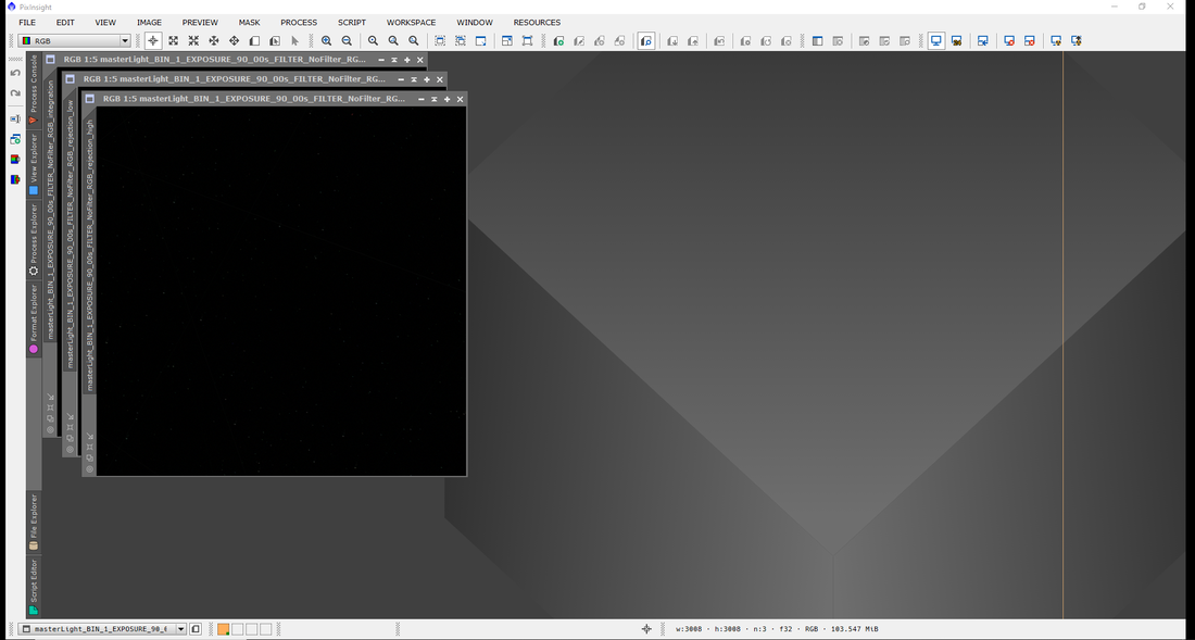
Fig. 1: Opening the file in Pixinsight after stacking in Pixinsight. Two of these files are part of the stacking process, stretching the images will show which is the picture, but usually the last file. If you stacked in DSS, the opening file will be a single file rather than three.
Screen Transfer Function
First, we need to stretch the image without actually stretching the image, so we can see the data in all its glory. Click on the process, all processes, and the Screen transfer function (shown in Fig. 2). it will open a box with several options on it. (Fig. 3)
Firstly click on the chain icon, this will unlink the RGB channels (there are other ways to process the unstretched image, but this way gives a better look and feel for the image and more colour) next click on the first image and then click the Nuke icon. This will auto-stretch the image so you can see what it would look like once finally permanently stretched. You are looking for a picture which resembles the target you aimed for (Fig. 4-6). If it doesn’t look or resemble the detail in Fig 5 close the picture.
Firstly click on the chain icon, this will unlink the RGB channels (there are other ways to process the unstretched image, but this way gives a better look and feel for the image and more colour) next click on the first image and then click the Nuke icon. This will auto-stretch the image so you can see what it would look like once finally permanently stretched. You are looking for a picture which resembles the target you aimed for (Fig. 4-6). If it doesn’t look or resemble the detail in Fig 5 close the picture.
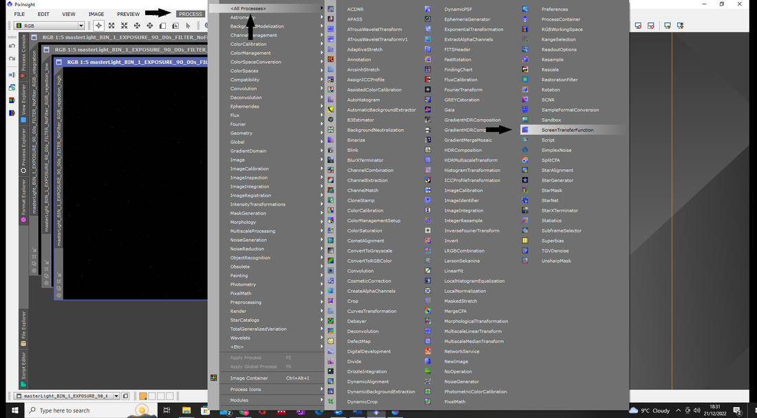
Fig. 2: Screen Transfer Function location.
|
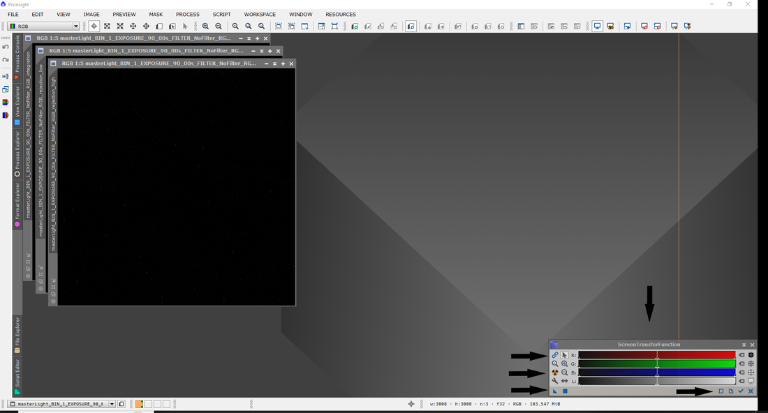
Fig. 3: Screen transfer Function options, with the arrows pointing to the main options
|
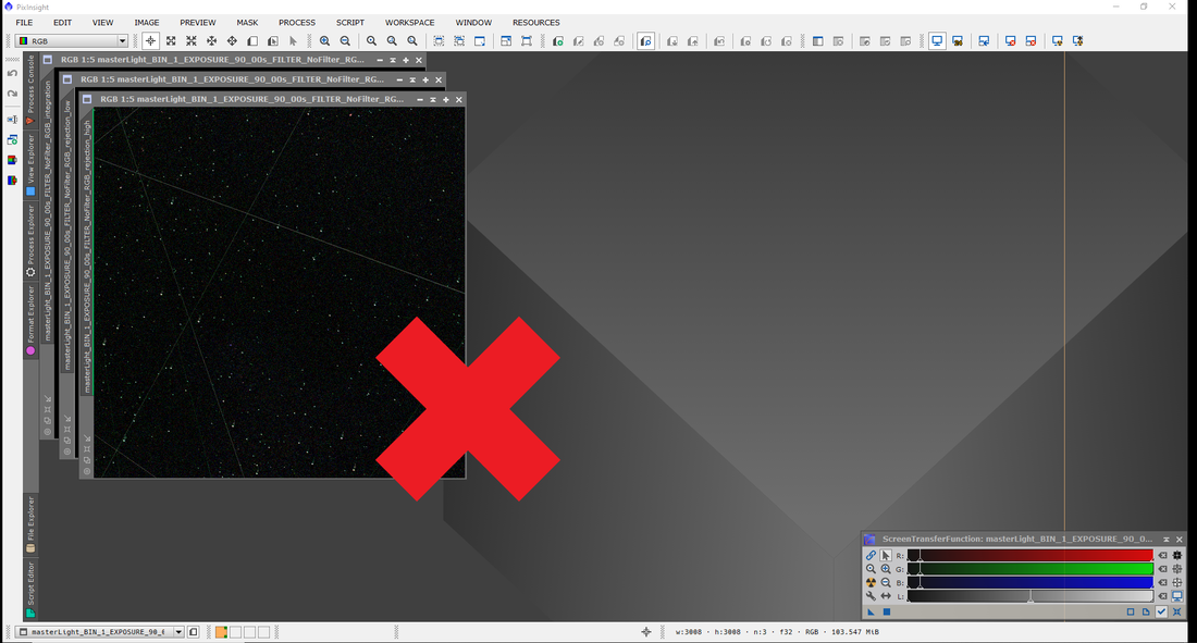
Fig. 4: Image stretch 1
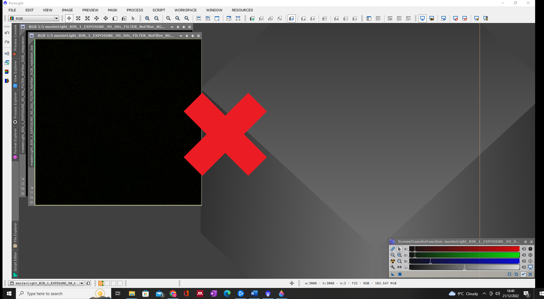
Fig. 6: Image stretch 2
|
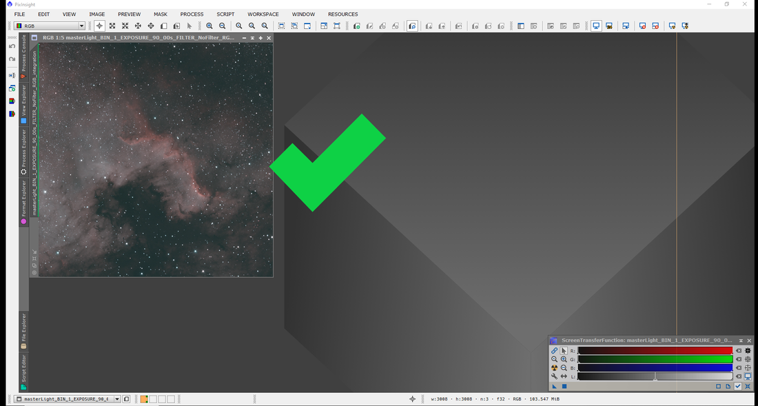
Fig. 5: Image stretch 3
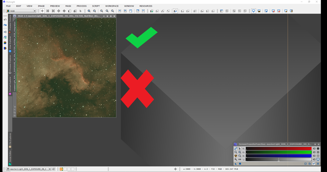
Fig. 7: Image stretch with linked channels. This is another method to process data but you potentially will lose a lot of the colour and the image will be predominantly red.
|
Fig. 7 shows what the picture would look like if the channels were linked. This will take a lot more processing and is unlikely to get the colour details out or be a lot harder to do.
EZ Denoise
Now we have the image temporarily stretched, it’s time to start processing the image. First, we need to remove some of the noise, using the EZ processing suite, Fig. 8. Click script, EZ processing suite, and EZ denoise.
A tab will open with a lot of information and options. Most of the options on here can stay as standard. But there are two options which you can choose from (Fig. 9) you can either choose Evaluate EX denoise Run or Run EZ denoise. The first option will process the image detail first and then you can choose how many iterations it uses to use while running the denoise. Or the second option is to just run it and it will run the basic denoise.
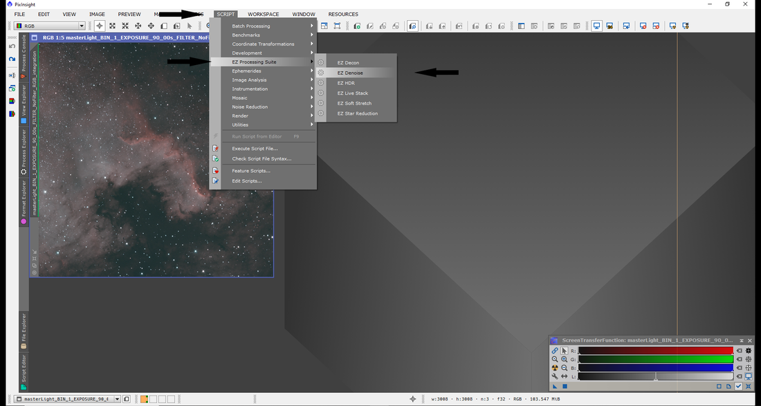
Fig. 8: EZ Denoise location.

Fig. 9: Two options with EZ Denoise. One for quick denoise and another for the in-depth process which will take longer.
The first option takes a while, as you are running the process twice. The second is faster with less denoise. Both look like Fig. 12 when the process is running, with Fig. 10 and 11 following the in-depth variant of denoise which finally will hit Fig. 12 for the final process. EZ denoise will create masks to run diagnostics through all three channels. This is the first part of the process and takes about 5-10 minutes. After the initial stage is done, it will show you the settings found from the evaluation. Move the iterations to max (5000) on the right-hand side and ‘run with these settings’ on the bottom right. Again this will take about 10-20 minutes.
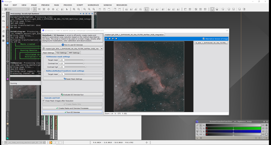
Fig. 10: Run denoise 1
|
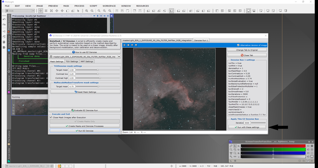
Fig. 11: Run denoise 2
|

Fig. 12: Run denoise 3
BlurXTerminator
Once complete, click the nuke button on the Screen transfer function to stretch the image post-denoise. Next, we need to use BlurXTerminator which is a deconvolution. This is a new program and worth the cost. Click on process, all process and BlurXTerminator (Fig. 13), this requires the use of a PSF Image, to figure out the size of the stars. PSF Image is fast, but you can create a preview to speed things up. (Fig. 14)
If you do not own BlurXTerminator, I'd suggest skipping this step for Nebula for the mean time. While it is possible, it does take a lot of testing in the options and numbers to get it right. There is a section for this in the galaxy processing page.
If you do not own BlurXTerminator, I'd suggest skipping this step for Nebula for the mean time. While it is possible, it does take a lot of testing in the options and numbers to get it right. There is a section for this in the galaxy processing page.
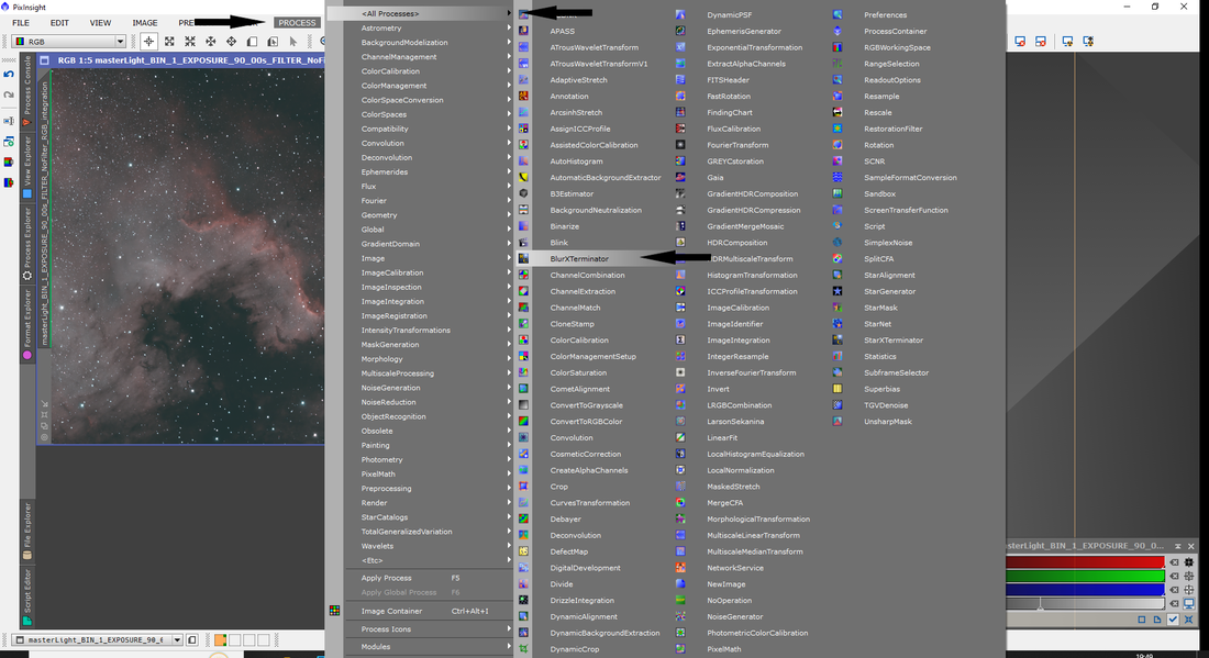
Fig. 13: BurXTerminator location
|
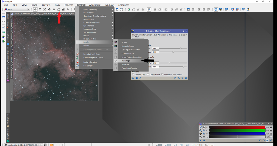
Fig. 14: PSF image location
|
Once opened, click Evaluate (Fig. 15) which will give you the Full Width at Half Maximum of the stars (FWHMx and FWHMy) simply add these together and divide by 2 to get the average of the two. Put this value in the PSF Diameter (pixels), click and hold the triangle and drag it to the image and let it do its thing. (Fig. 16)
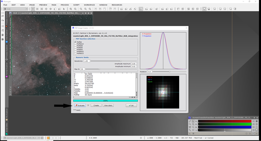
Fig. 15: PSF image process to find out the size of the stars. This can be done directly to the picture or can be done in a preview which will make the process faster.
|

Fig. 16: After the PSF is known and installed, drag and drop the triangle onto the picture and let it run its process.
|
Histogram Stretch
Once this is complete, you are ready to stretch the image. This is quick and simple. You need the Screen Transfer Function and the Histogram Transformation (process, all processes, histogram transformation - Fig. 17). Simply drag the triangle from the Screen Transfer Function to the Histogram transformation (Fig. 18) and then simply drag the triangle from the Histogram transformation to the image. If done correctly, the image will turn white. Simply click the ‘reset screen transfer function’ (Fig 19 & 20), after this the image is permanently stretched and we can continue with processing by stretching the image using curves etc.
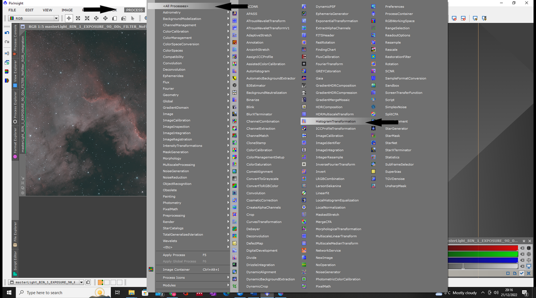
Fig. 17: Histogram Transformation location
|
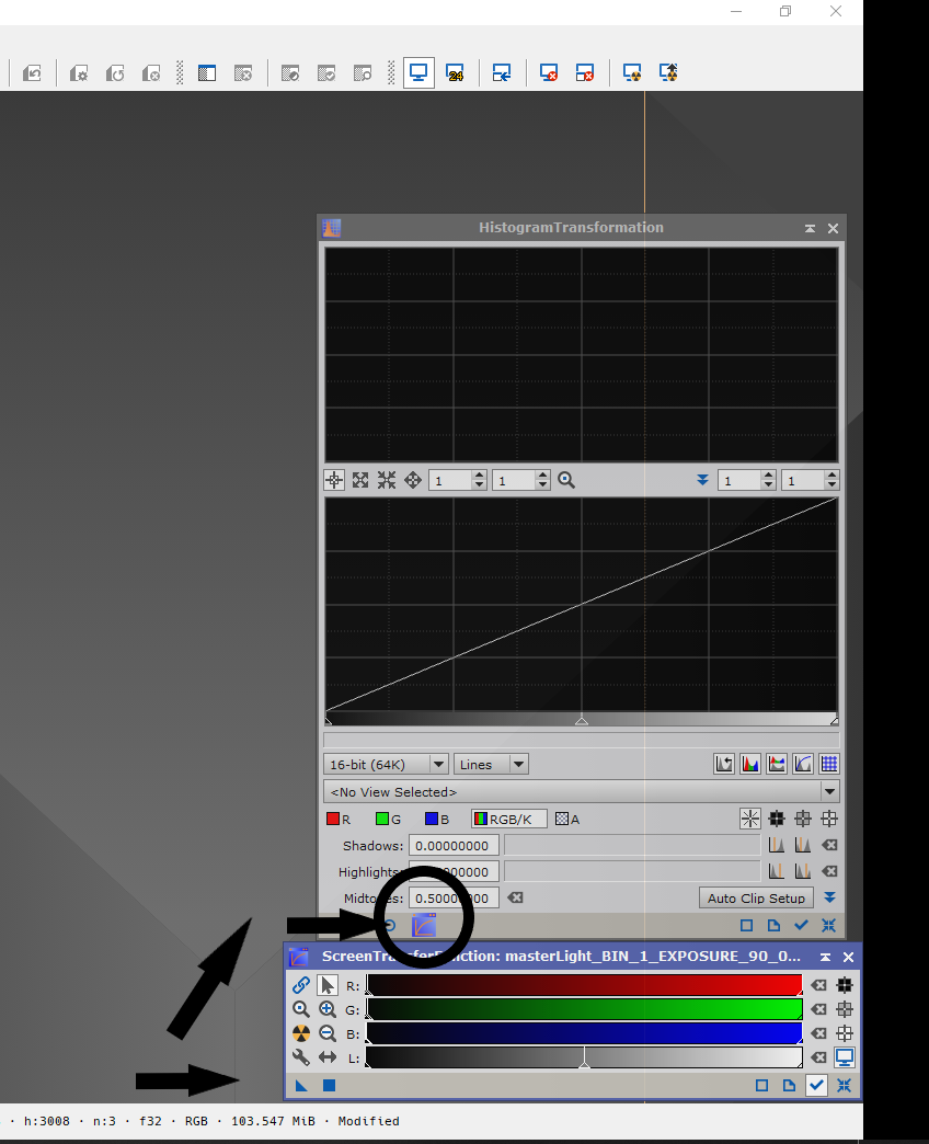
Fig. 18: Histogram Transformation and Screen Transfer Function. Drag the triangle from the STF to the lower bar on the HT which creates the curve on the HT ready to stretch the image.
|
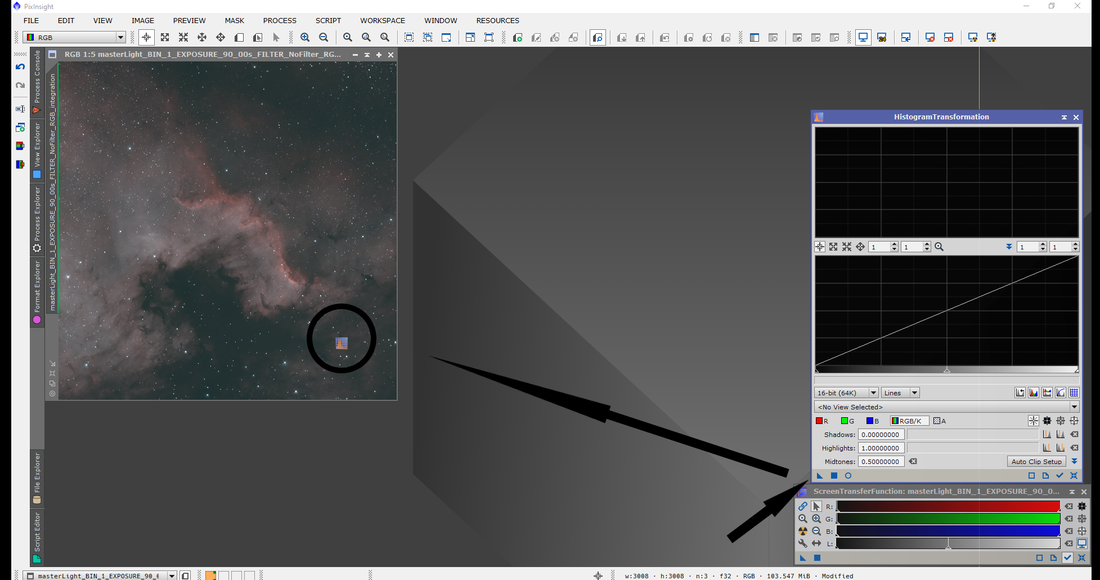
Fig. 19: Dragging the pre-stretched HT to the image to stretch the image from the STF.
|
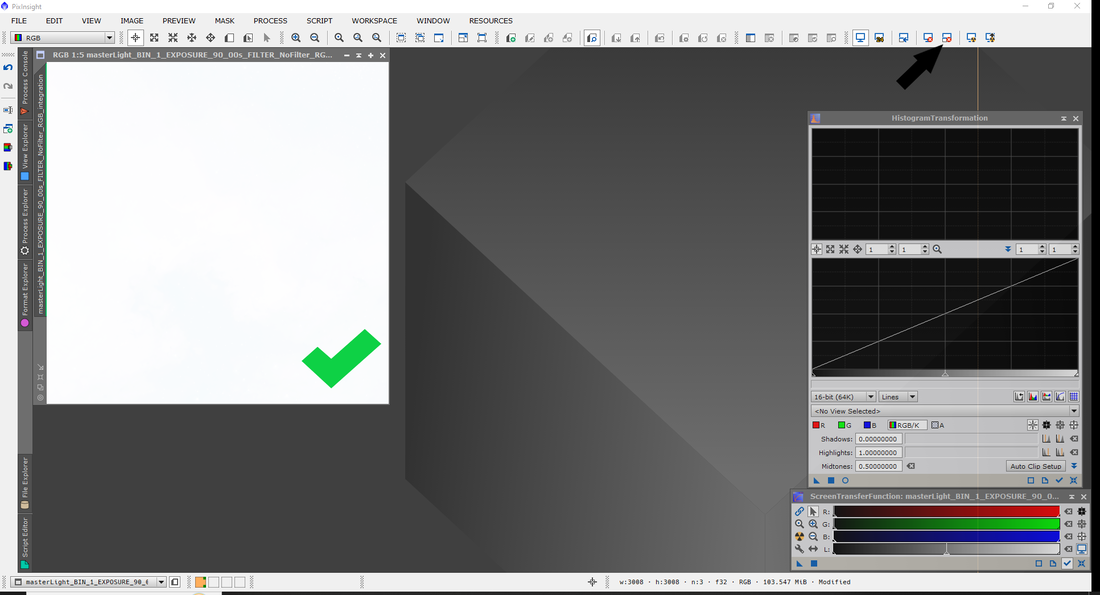
Fig. 20: Stretched image. This will be a white image as the image is going from the HT. Simply click the cancel stretch button to see the permeant stretched image.
|
Dynamic Crop
Time to crop the image. This will remove any artefacts from capturing the image during the night from dithering. This is easy to do. Open Dynamic Crop (Process, all processes, Dynamic Crop) this will open the Dynamic crop option. The quickest and easiest way is to click on the image, hold the mouse button down, make a shape you want to crop to, and simply hit the enter key. This will remove the outside of the chop you created and move any artefacts from stacking, etc., as seen in figures 21-25.
This can be done before or after star removal. if you are doing this after the stars are removed then you need to drag the triangle to the star image as well as the starless image. so both the starless and star images are both the same size (do not reset the Dynamic crop before both images are set)
This can be done before or after star removal. if you are doing this after the stars are removed then you need to drag the triangle to the star image as well as the starless image. so both the starless and star images are both the same size (do not reset the Dynamic crop before both images are set)
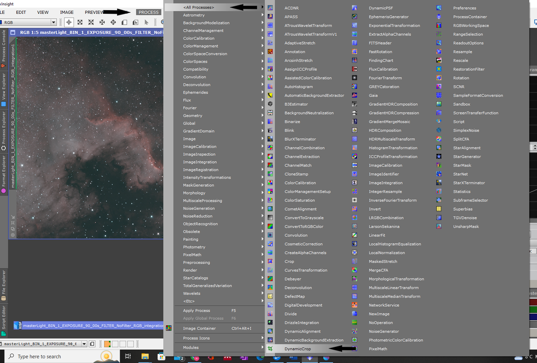
Fig. 21 Dynamic Crop location.
|
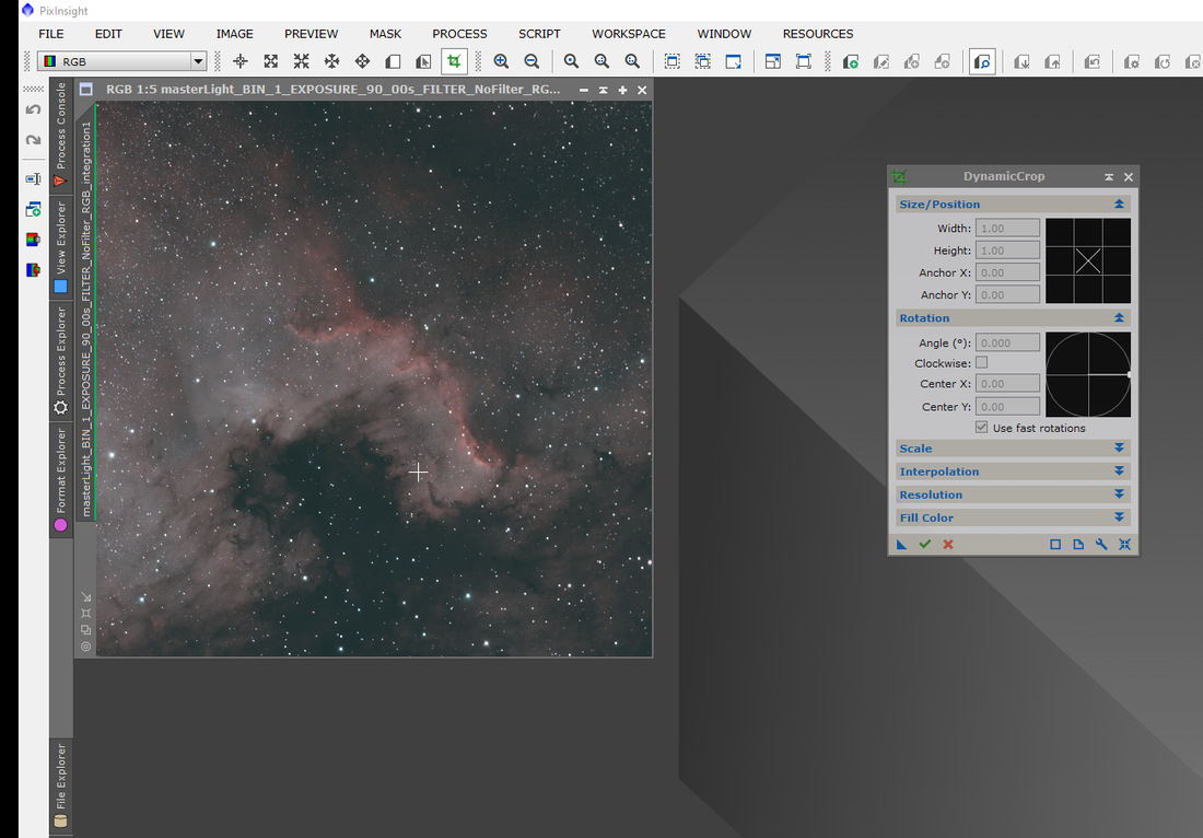
Fig. 22: Dynamic Crop box details.
|
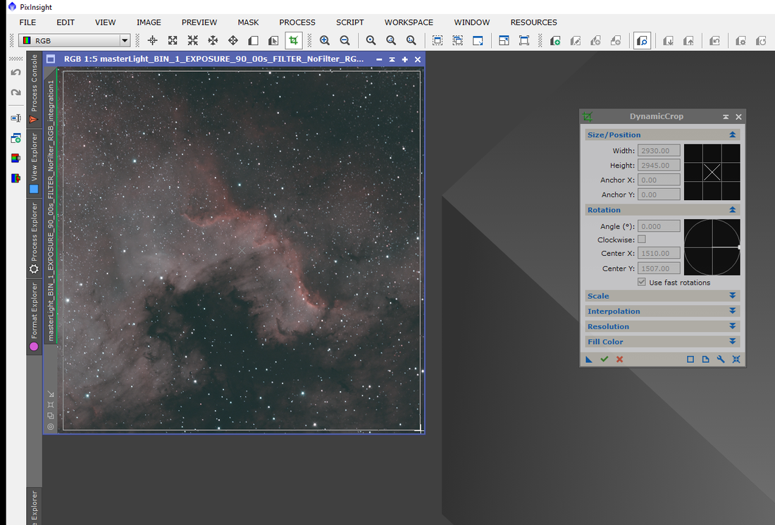
Fig. 23: Simply click the tick in the bottom left or drag and hold the cursor over the picture to draw the box. This box is adjustable and customizable.
|
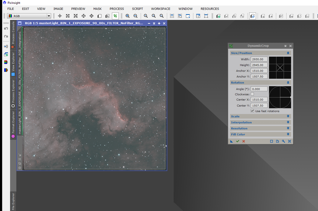
Fig. 24: Once you are happy with the crop box, hit enter and the crop will cut the picture to the box.
|

Fig. 25: Finished cropped picture.
Star Removal
|
Before we stretch the image with curves, we need to remove the stars.
The stars are prone to bloating when stretched, so we need to remove them early as possible to avoid this. For this, we will use the StarXTerminator add-on found in Process, all processes, StarXTerminator (Fig. 26). StarXterminator box will pop up with a few options. Click select AI and click StarXTerminator.11.pb and then click open (Fig. 27). The options box will shut and it’s a case of dragging and dropping the triangle onto the image (same as before, which can be seen in Figs 28-30). |
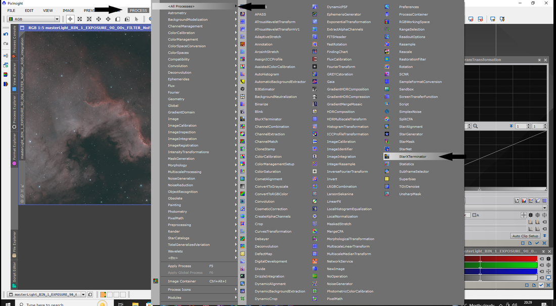
Fig. 26: StarXTerminator location.
|
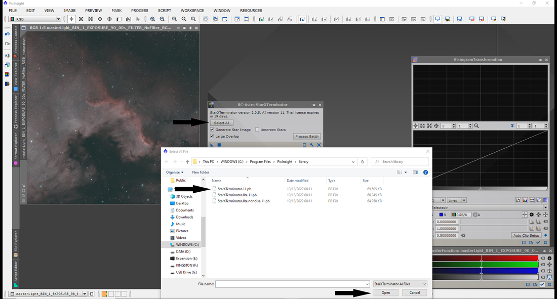
Fig. 27: Clicking file AI button, which on the file StarXTerminator.11.pb and click open. This setup the software ready to be used in StarXTerminator.
|
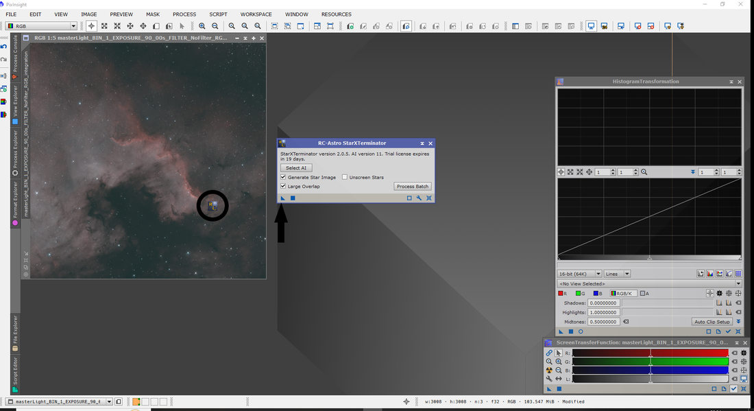
Fig. 28: starXT3
|
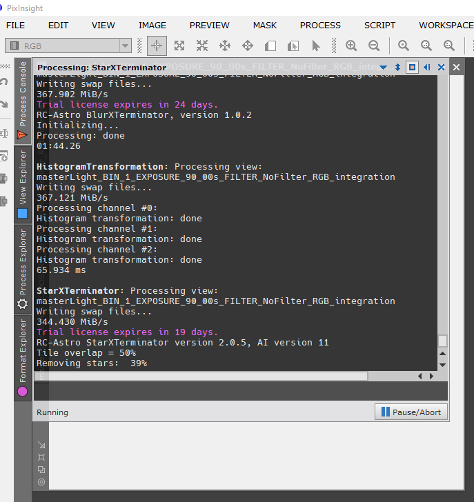
Fig. 29: starXT 4
|
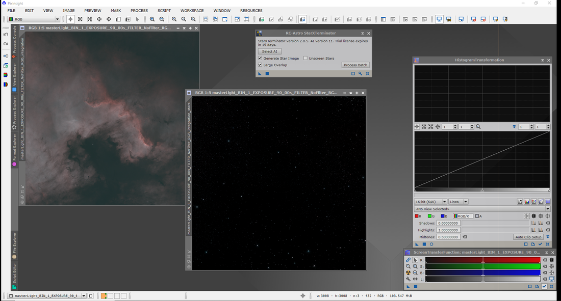
Fig. 30: starXT 5
|
If you do not own StarXTerminator, there is a PI version called Star Net which will do the same thing but not necessarily as clean as StarXTerminator (Fig. 31). Once Starnet is open you may need to locate the weight files for removing the stars. Click the spanner which will open the preferences. If the two locations are empty, you will need to locate these files before being able to use Starnet. (Fig 32) Click on the file icon and go to Windows C: - program files - pixinsight - library. Click on the relevant file related to the weight (RGB with RGB and Mono with Mono) and click open. Do this for both file locations. Once these are in place drag and drop the triangle onto the image.
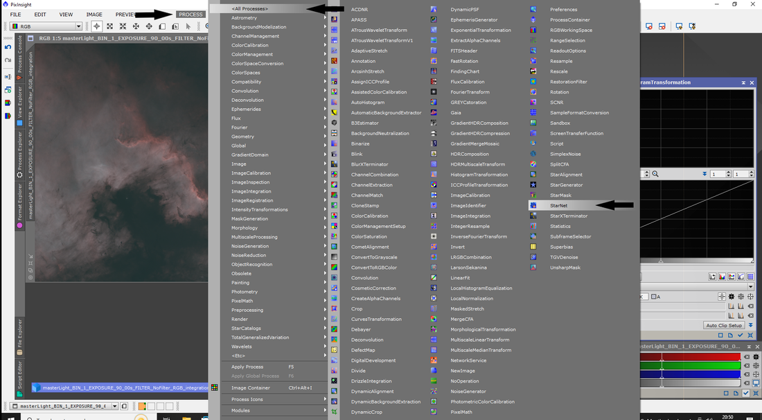
Fig. 31: star net
|
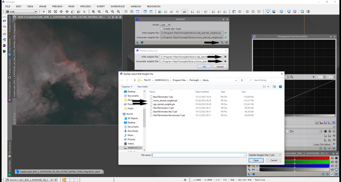
Fig. 32: star net 2
|
Renaming the star image
Before we move on to processing the nebula, we need to rename the star image later on. Currently, it’s named - masterLight_BIN_1_EXPOSURE_90_00s_FILTER_NoFilter_RGB_integration_stars – we need this shorter. Open the star image and double-click on the name and a box will appear which will allow you to change the name. (Fig. 33) The blue text will be the new name. simply change it but it needs to be simple – I use star_mask. Once you name it click ok (Fig. 34 & 35).
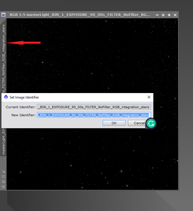
Fig. 33: Name change by double clicking the name tab which opens this tab.
|
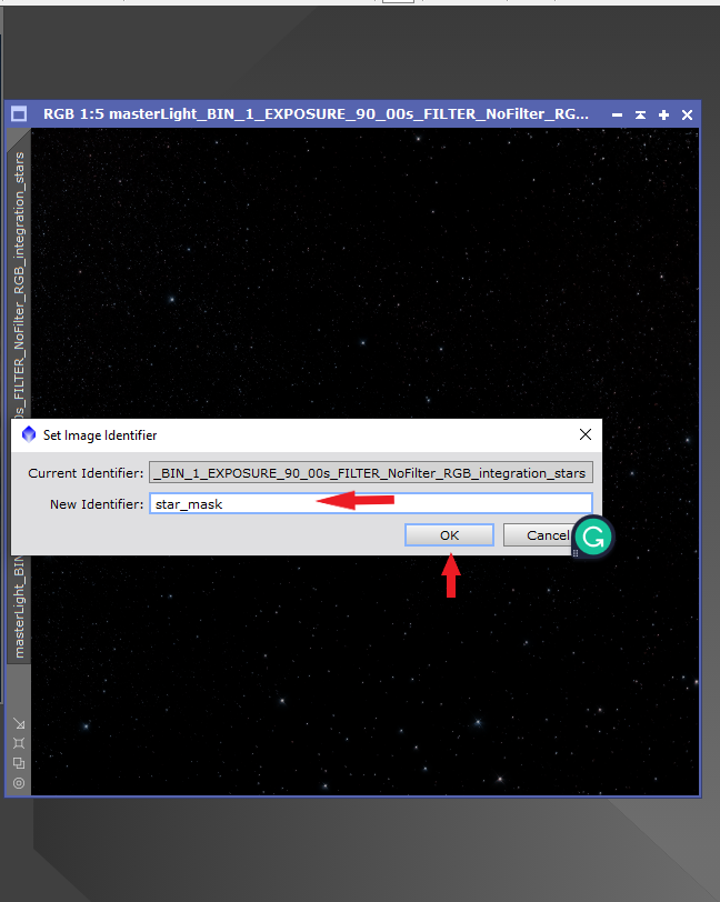
Fig. 34: name changed to star_mask
|

Fig. 35: Finished name change of the stars.
Removing the Green - SCNR
Now the stars are removed we can process the nebula, without the worry of bloating the stars. But first, let’s make sure we have removed all the green colour from the image using SCNR (Process, all processes, SCNR - Fig 36) This part is quick, it is choosing the amount in decimal points of how much green you want to remove (1.00= 100% and 0.9 = 90% etc) and then drag and drop on both the starless image and star image to remove the green, Which is seen in Fig. 37. Depending on the target and image, this may or may not have any effect.
This process can be done before or after removing the stars and is personal to you. Do whichever is easiest for you during the process but must be done after you have stretched the image. If you choose (or like me, you forgot...) to remove the green before you remove the stars, don't forget to remove the green from the star image also.
I generally remove all green from the images, but you can choose how much you take out of the image. Have a play with percentages and reset the green and have another try with a different percentage.
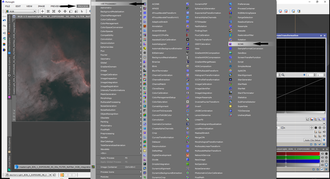
Fig. 36: SCNR location.
|
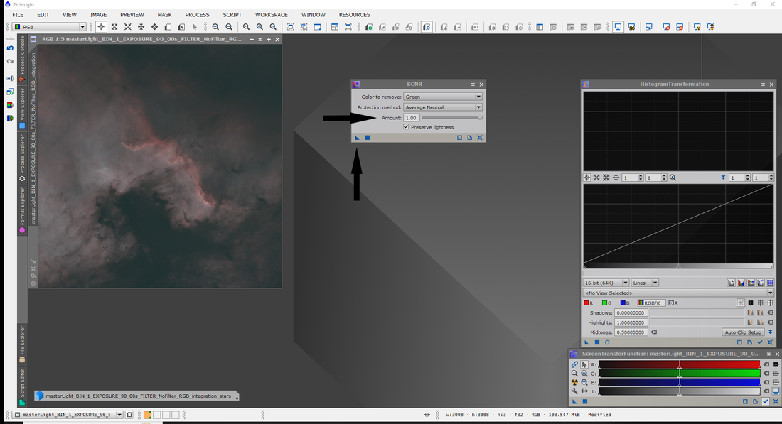
Fig. 37: Applying the SCNR to the image, using your own preference percentage of green you want to remove.
|
Stretching the image
Moving on to the curves and colours. Both of these are variables and dependent on personal liking. This part is more experimental till you find the right colour and contrast. First, curves. Open up Curves Transformation (process, all processes Curves Transformation) (Fig. 38) and this will open a box with a linear line graph and several options at the base.
First, we will concentrate on RGB/K channels. This channel may be pre-set when you first open it, if not just click it so the white box covers RGB/K. We are going to create an S curve in the graph by moving the line. We aren’t worried too much about the graph, but more about the image and how it reacts. (Fig. 39)
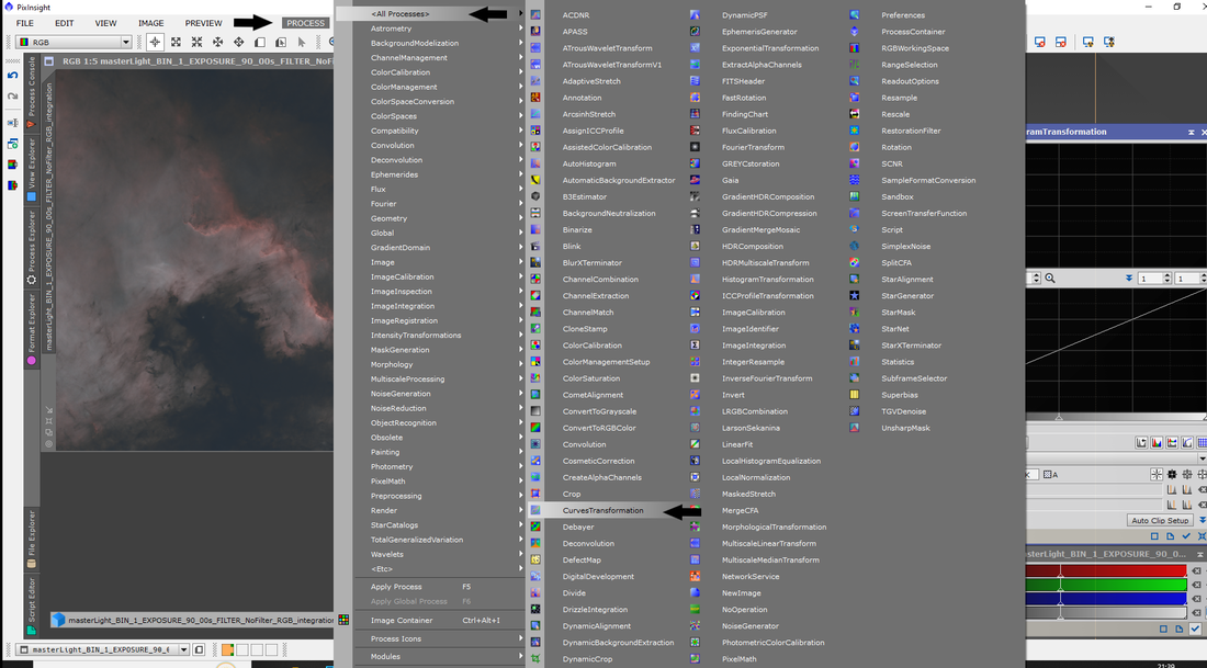
Fig. 38: Curves Transformation location.
|
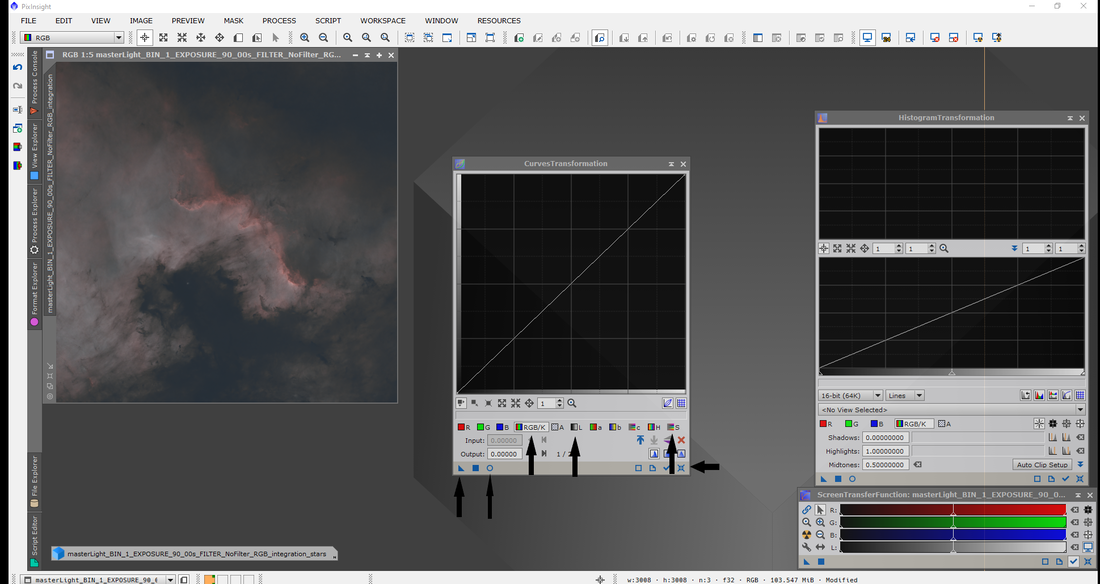
Fig. 39: Curve box details.
|
First, we open a preview window, this will allow us to see what will happen to the image before we apply it permanently to the image which is located in the bottom left hand corner (third on the right of the three buttons - Fig. 39 and 40). After we stretch the image to a permanent state, we always use preview. It is better to see what we are doing before we do it. Saves undoing things. Click the circle icon at the bottom left of the curve’s transformation box. This will bring up a new window and will show you what will happen to the image if we do it to the image (Fig. 40).
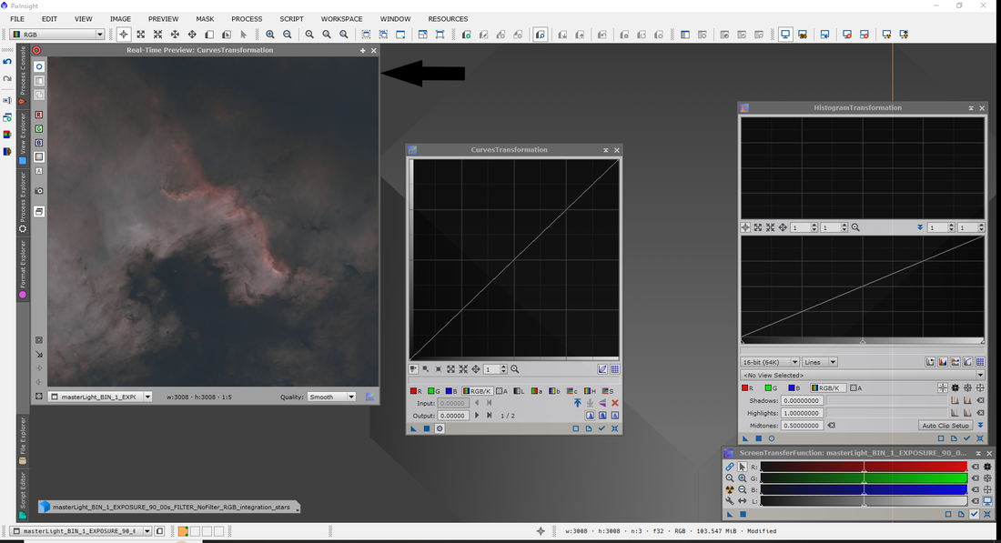
Fig. 40: Curves preview.
|
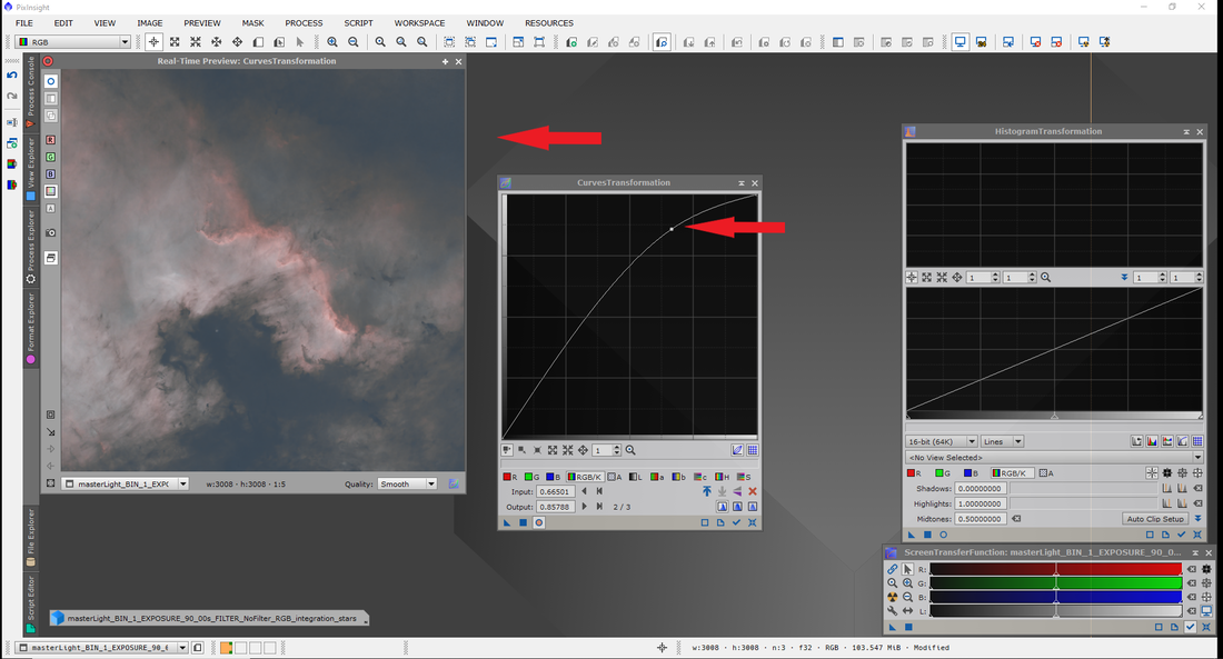
Fig. 41 Moving the line increasing the RGB/K. Upper part of the line is the foreground and the lower line is back ground.
|
Now click on the upper part of the line in the curves transformation and move it up. Watch what happens to the preview, this will be your indication of how much you can push the data (Fig. 41). Now do the same to the lower part of the line and pull it down, remember it is a personal choice on this. This part you can play around with this to try and understand what happens to the nebula and background when you push the curve (Fig. 42).
Once you are happy with the curves, close or move the preview tab and drag and drop the triangle to the main picture to apply the curve to the picture (Fig.43). This can be applied multiple times if required and to compare the image to the previous version, click the circle button on the curves transformation so the colour is removed from the central part of the circle to see what it is currently to what the change will do to the image if applied.
Once you are happy with the curves, close or move the preview tab and drag and drop the triangle to the main picture to apply the curve to the picture (Fig.43). This can be applied multiple times if required and to compare the image to the previous version, click the circle button on the curves transformation so the colour is removed from the central part of the circle to see what it is currently to what the change will do to the image if applied.
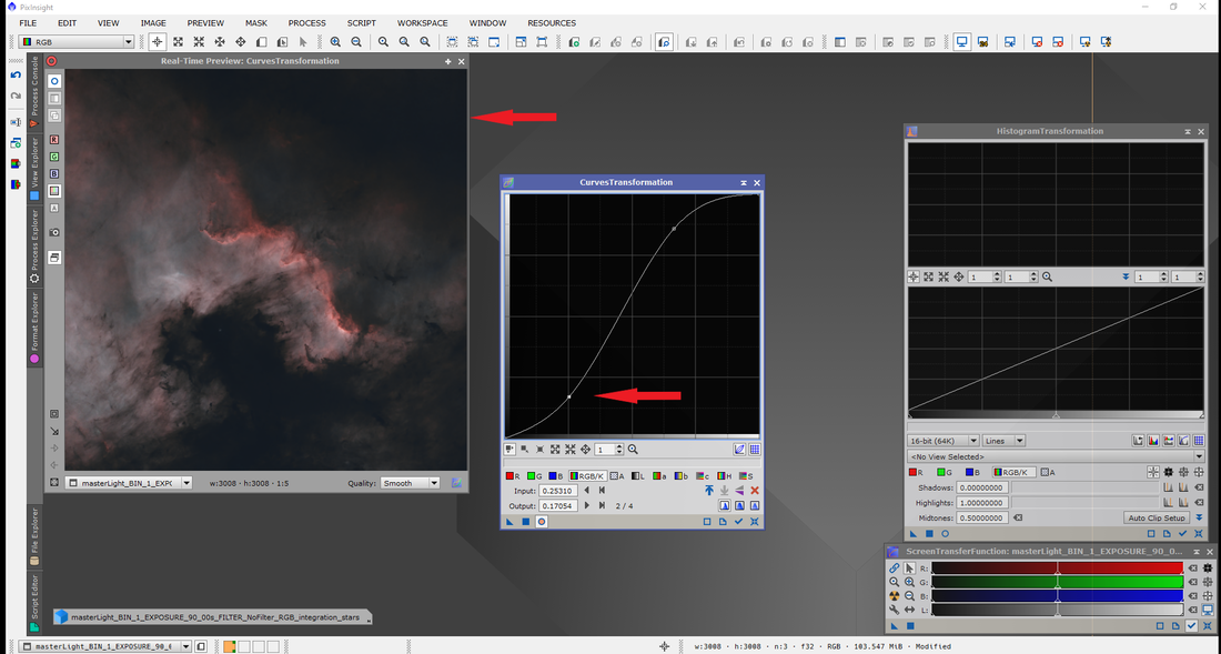
Fig. 42: Pushing the lower part of the line which darkens the background of the picture. Comparing Fig. 42 and 41 shows a clear difference between them.
|
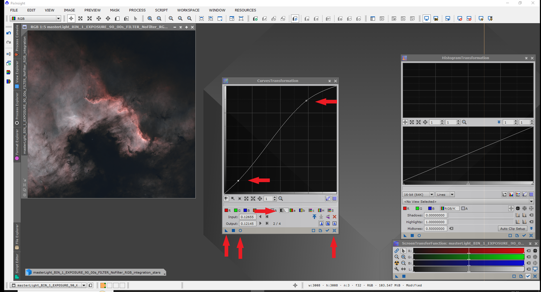
Fig. 43: Moving to the Luminance channel. Click the L button marked by one of the red arrows and reset the line (if the line isn't reset it will push the previous channel used again). Reset is the bottom right-hand button, marked by the red arrow.
|
Time to move on to the Luminance part of the curves. Hit reset at the bottom right (x style in the image, See Fig. 43) this will reset the curve graph to a straight line. Click on the L to the right of the RGB/K button so the white box surrounds it and again hit preview. You will find that you won’t need to do too much with luminance, but slight adjustments will make a difference. As before, click and hold the line making a slight S curve. Once you are happy with the changes, apply them to the image (Fig. 43).
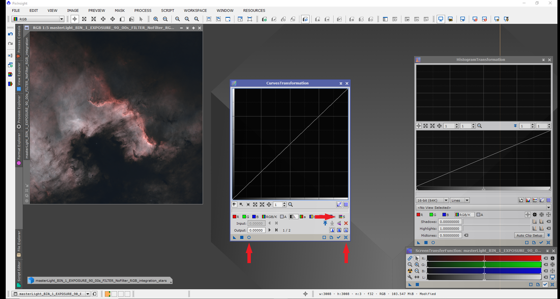
Fig. 44: Saturation stages of the process. Reset the graph, select Saturation and use the preview.
|
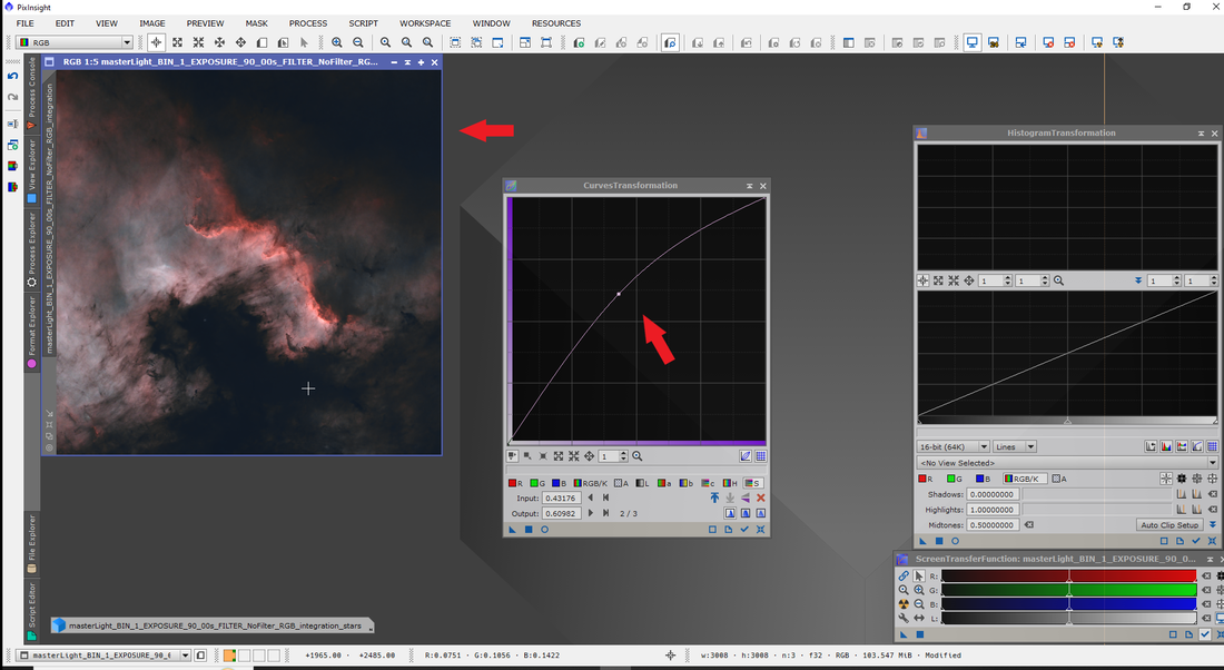
Fig. 45: adjusting and applying the curve.
|
Saturation is a big part of the processing as it will change the colours of the Hydrogen and OIII data. Reset the data and click the S which is on the right near enough above the reset button. Again using the preview, we will adjust slightly the colours of the nebula itself but instead of a curve, we are just pulling the centre of the line to the upper left till you are happy with the colours and then drag and drop onto the image. Since we are hitting mainly the Hydrogen, we will use another process after this part. (Fig. 45)
Colour Saturation
Minimise or close the Curves Transformation window as we won’t need it unless we want to adjust later. (top right corner). Now open Colour Saturation, which is in Process, all processes, Colour Saturation. (Fig. 46) This will open a different type of graph, one which is horizontal but with no line. Now click on the central line and make a point through the colours (Fig. 47) We are primarily after Oxygen (blue) over red.
To find where the colour is, hover the cursor over the Image and a plus curser will form click and hold and move over the image, you will find what the colours are as it will appear on the Colour saturation graph, giving you an idea where the colours are and what colour is there (Fig. 48).
To find where the colour is, hover the cursor over the Image and a plus curser will form click and hold and move over the image, you will find what the colours are as it will appear on the Colour saturation graph, giving you an idea where the colours are and what colour is there (Fig. 48).
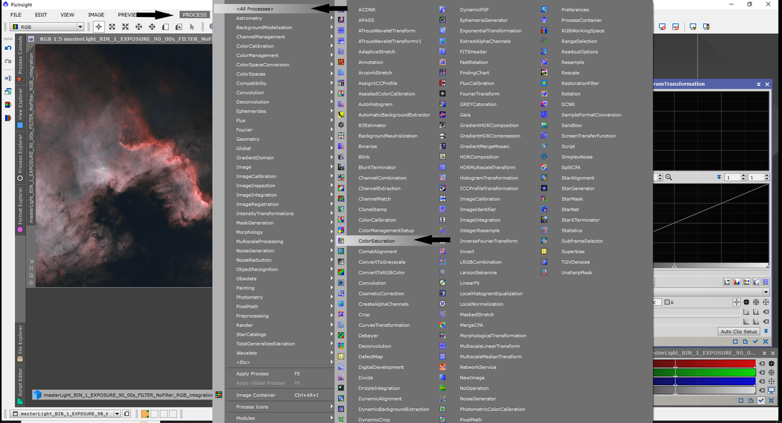
Fig. 46: Colour Saturation location.
|
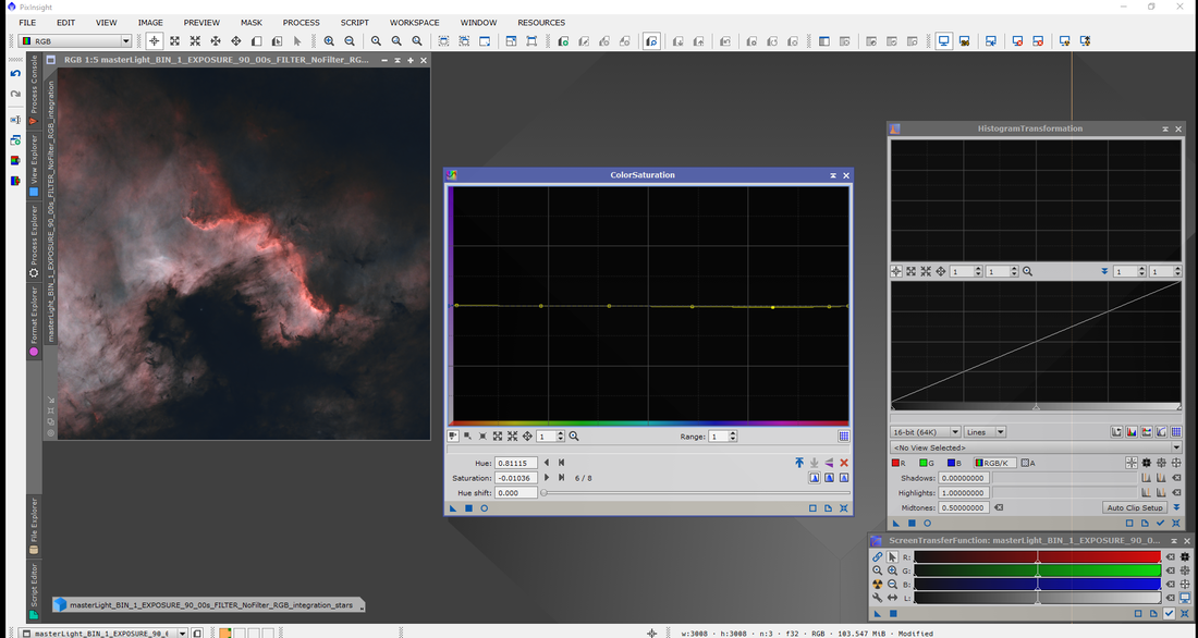
Fig. 47: Prepping the graph. Click on the central line from one side to the other, creating about 5-6 dots.
|
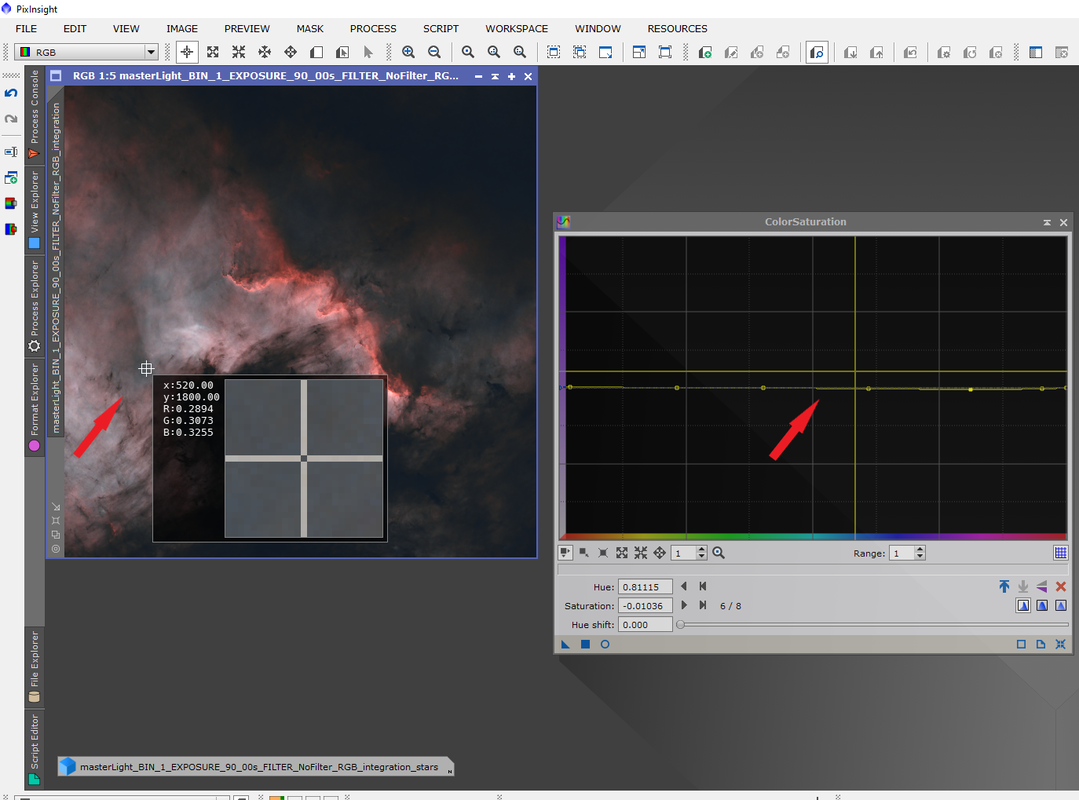
Fig. 48: Colour location. Click on the preview to bring up a larger box showing colour details. In turn this will bring up on the graph where the colour is situated on the graph. You are looking for primarily OIII (blue colour) and red secondary (since red can be pushed with the saturation in the Curves Transformation.
|
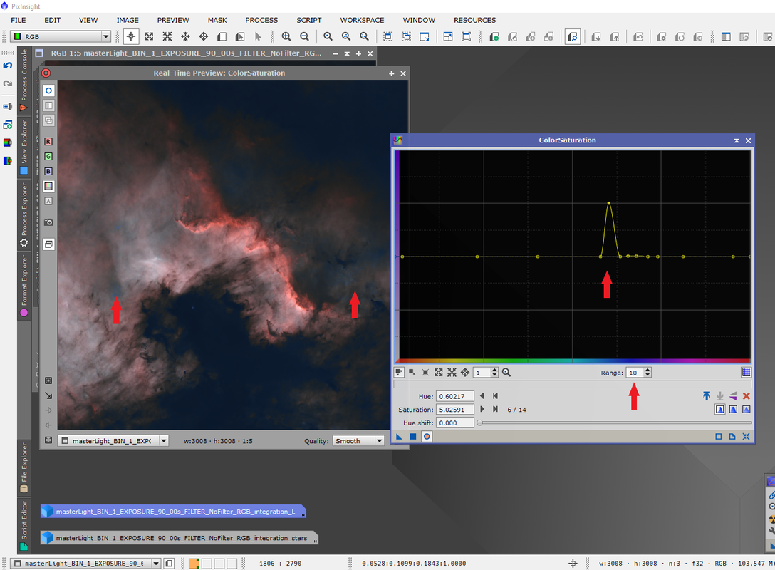
Fig. 49: Saturation of the blue. If you are using a mask for this part increase the range. I sometimes find leaving the mask off and adjusting the histogram slightly better.
|
Find the blue colour on the graph and place a point on the central line for this colour then place points on either side of this point so the curve will be quite tight, then drag the middle point up the graph with the preview open until you are happy with the result. If you find you reach the top of the graph, click on the range arrow to make the number rise to 3-4 (maybe higher if you feel the colour isn’t coming though. Make sure the location has Oxygen in the area before trying to push the blue too much, or it will just push the background colour which isn’t what the aim is here. (Fig. 49)
Dark Structure Enhance
You can do two more things to this image before putting the stars back into the image. Dark structure enhance, and HDR. Both are optional and both are worth looking at in case it has a notable change to the final image. Masks can be used here also, but with the stars removed, it isn't always essential.
Dark Structure Enhance is a tool which is quick and simple. (Script, Utilities, Dark Structure Enhance) (Fig. 50). The main parts of this are Iterations, amount, and layers to remove. Start with the base figures, click ok and see how it looks. The undo button will be needed here due to removing the dark structure enhance from the image as there is no preview. (Fig. 51-53)
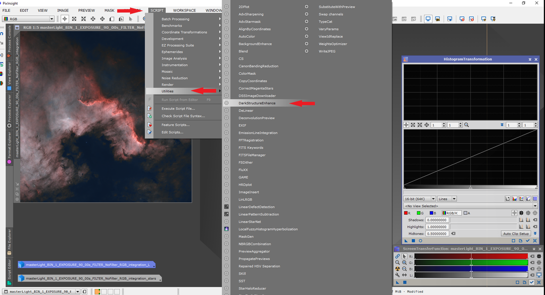
Fig. 50 DarkStructureEnhance location
|
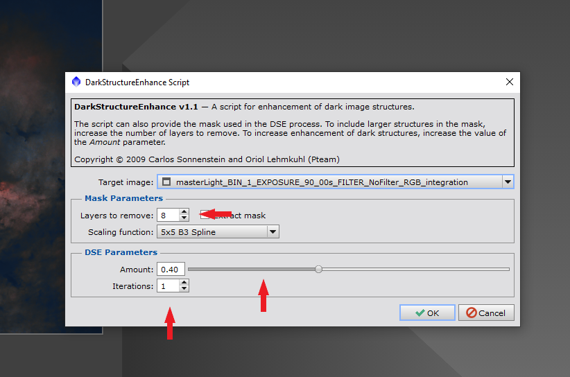
Fig. 51: Dark Structure Enhance options, keep in mind there is no preview.
|
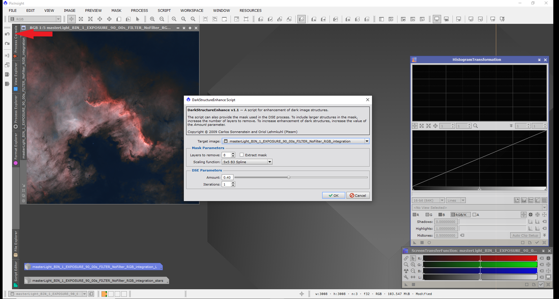
Fig. 52: Use pre-set options, reset and adjust the options and reapply. Keep doing this till you are happy, or you click on the pre-set was best.
|
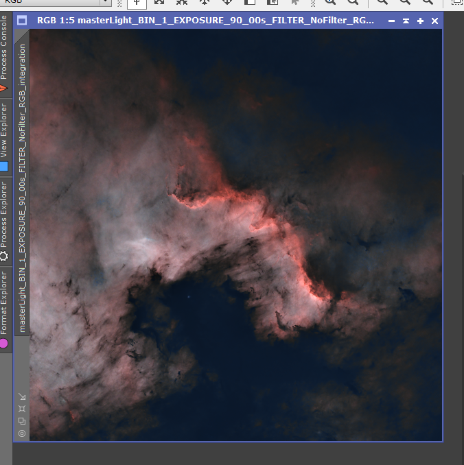
Fig. 53: Final out come of Dark Structure Enhance. Dark parts of the picture are darkened to give the picture more depth.
|
HDR
HDR (Script, EZ Processing Suite, EZ HDR - Fig 54) is a script which is hit and miss depending on the target. Sometimes it will make a difference, other times next to none. Again this script is trial and error, but I generally leave it as basic settings and go from there. Adjust the settings and click ‘run EZ HDR’ this will create masks necessary for the process and create a new Image with HDR in the name. Click to Open and compare. HDR is good for bright objects, such as Orion nebulas core and Galaxy cores. (Fig. 55)
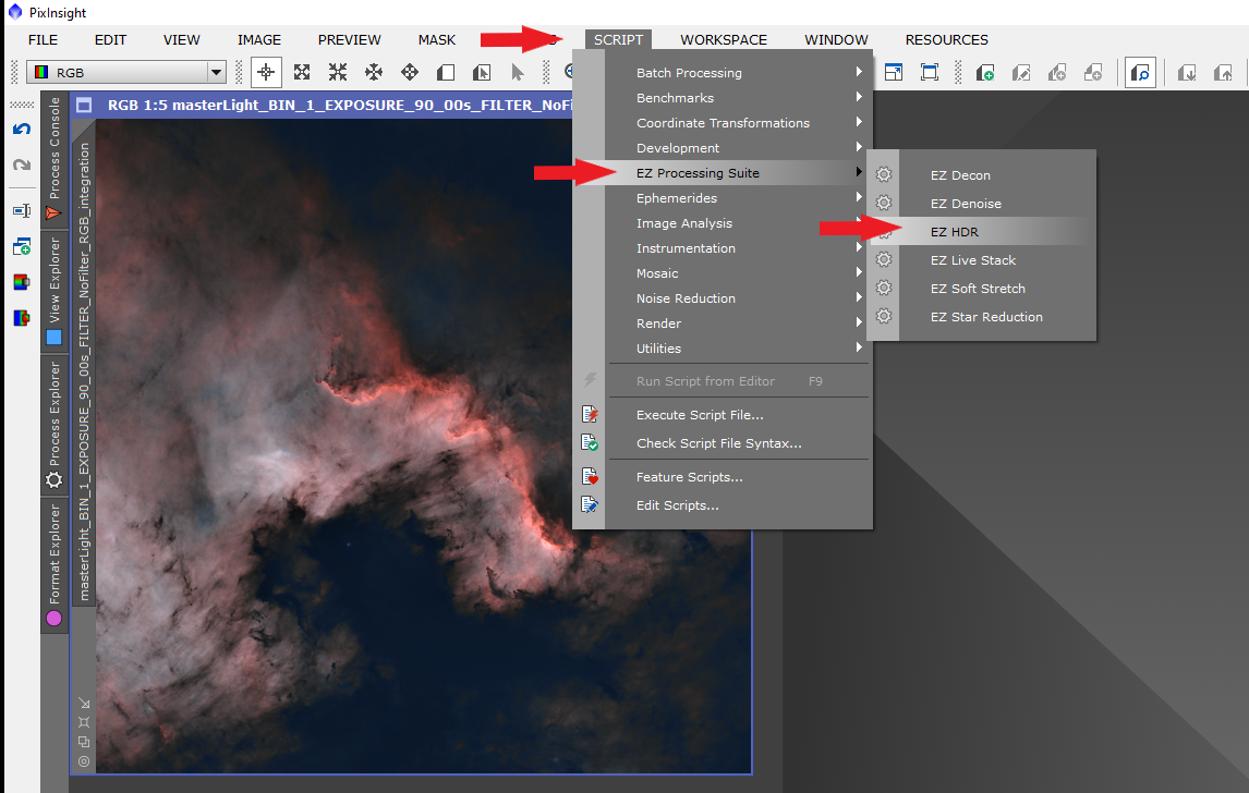
Fig. 54: HDR location.
|
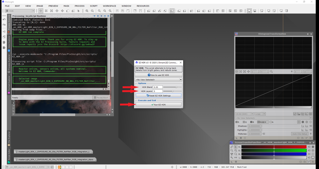
Fig. 55: HDR options. Again, like DarkStructureEnhance, this doesn't have a preview as it creates a new picture altogether. The new picture will be named the same as the originally named picture but with _HDR at the start or at the end.
|
Revisiting Curves
Now is the time to go back to curves if you fancy changing any of the details, you can increase or decrease curves by playing with the curve on the preview. It’s good to play and test this curve as it is a powerful tool to have for processing images. See the section on curves above.
Pixelmath and adding the stars back to the image
It is now time to move the stars back into the image and apply star reduction to the image. Open PixelMath (Process, all Processes, PixelMath) (Fig. 56). This tool is used for a lot of things including adding images together as well as merging images in percentages. (another tutorial)
The line you need for this is this $T + star_mask (Note the spaces between $T + star)
(the star_mask is what we discussed earlier in the tutorial, if you named the image to something else, then put that in place of star_mask.)
Once you put this in the PixelMath simply drag the triangle to the nebula image for it to combine the image. (Fig. 57 & 58)
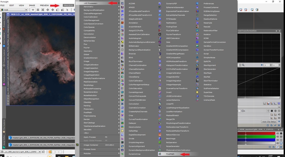
Fig. 56: Pixelmath location.
|
Fig. 57: Applying pixelmath to the image to reapply the stars to the image.
|
Fig. 58: The completed combination of starless and star_mask image using Pixelmath.
Star Reduction
Finally, time for star reduction. Depending on the image, it may not need reduction. But if you find your image with large or bloated stars then this would be essential. Open EZ star reduction (Script, EZ Processing Suite, EZ star Reduction - Fig. 59).
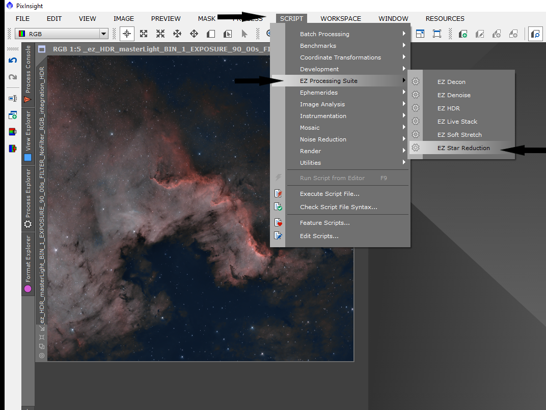
Fig. 59: EZ Star Reduction location
|
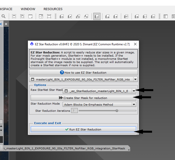
Fig. 60: star reduction 2
|
There are several options. One you can just click Run Ez Star Reduction and it will create all the masks for you, or you create a mask ahead of starting the process. Both ways end up with the Ez Star Reduction creating what it needs for it to process the stars. This process is fast and after it has finished the processing is complete. If you are unhappy with the process of reduction, just click the undo button in the top left corner of Pixinsight just below the file button. (Fig. 60)
Saving the image
Time to save the image. Click the file in the top left-hand corner of Pixinsight and click ‘save as’ (Fig. 61)
It is important to make sure the name reflects the images, so you know what you did on this image and what the data collection etc. (if you processed the picture from DSS you won’t need to change the name, but if you stacked the image in Pixinsight, you would need to change it to. Also, think about if you have processed this image before but haven't added any new data. Maybe Add V# E.G., V2 or V3 depending on how many times you have processed this image.
Name of target_total exposure_sub-exposure time_scope_camera. So for example this one would be NGC7000_81mins_90sec_RASA8_533mc
Anything which was placed in form of the name of the target needs to be removed from the start of the file is the name of the target.
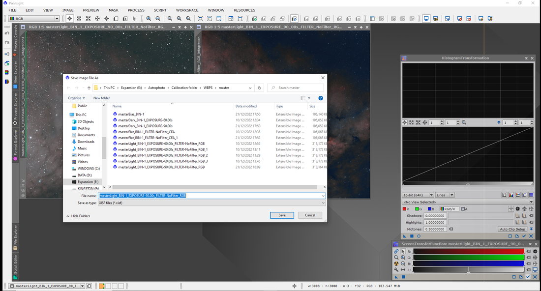
Fig. 61: Saving the picture. Choose your preferred location and click Save.
Congratulations – you have successfully processed an Image using Pixinsight. I hope this has helped you and that you keep striving to improve your images. The more you process, the better you become.

NGC 7000 starting picture with the basic stretch.
|
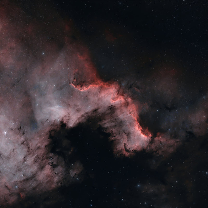
NGC 7000 final picture.
|